


Productivity is simple to define but tricky to calculate. In economics, it represents the ratio of what you produce to what it takes to produce it. Think of it as a scorecard for efficiency. You take the total output of a specific category of goods and divide it by the total input required, such as labor or raw materials. The result is an average that tells you how much value you get back for every unit of resource you put in.
You can plug almost anything into the denominator of this equation. It does not have to be just people. You can measure the productivity of land, capital, or specific types of fuel. You can even combine inputs to see how labor and capital work together. When you look at all factors combined, you are dealing with total factor or multifactor productivity. Changes in this specific metric over time show you the net saving of inputs per unit of output. It represents the increase in productive efficiency.
Economists sometimes call this the “residual.” Why? Because it captures the portion of output growth that you cannot explain by simply adding more measured inputs. It is the mystery part of growth. Meanwhile, partial productivity ratios look at output against a single input. These ratios are messy, though. They reflect changes in efficiency, but they also show substitution. For example, if you replace labor with capital goods or energy, the ratio shifts. That change is not just about getting better; it is about switching what you use.
Why labor dominates productivity measurement
Labor is the most common factor used in productivity calculations. It is the default choice for two main reasons. First, labor costs make up a relatively large share of the value of most products. Second, counting people is easier than measuring capital.
If you just count heads, you ignore skill differences and work intensity. But that is often all you can easily do. Statistics on employment and labor-hours are readily available. Data on other productive factors is often hard to obtain. This creates a bias. The term “labor productivity” does not mean labor is solely responsible for changes in the ratio. Improvements in output per unit of labor can come from better human efficiency, yes. But they can also come from machinery, technology, or other variables.
There is a deeper reason for the focus on workers. Human beings are both the means and the end of production. We produce things, but we also consume the standard of living that production creates. That dual role makes labor productivity a central metric for understanding economic well-being.
The shifting role of land and capital in economics
Land productivity used to be the big one. In ancient and preindustrial times, the products of the soil were the bulk of total output. If your soil was low-yield, you were poor. That connection between land and standard of living was direct. Today, that link is weaker. We no longer believe a country’s economic well-being is inevitably tied to the productive powers of its land.
Modern agricultural methods have expanded the productive potential of soil. It is not fixed. Industrialization has also reduced people’s dependence on agriculture. Trade opportunities have allowed countries with meager agricultural endowments to overcome those handicaps. You do not need rich soil to be wealthy if you have trade and industry.
Capital productivity is a different story. Economists have been interested in plant, equipment, tools, and other physical aids for a long time. But actually measuring it is a recent development. Improved statistical reporting and data availability in advanced industrial countries, especially since World War II, have encouraged systematic efforts. Progress has been limited compared to labor productivity. The theoretical and practical difficulties are considerable.
“The residual reflects that portion of the growth of output that is not explained by increases in measured inputs.”
How to interpret productivity data for better decisions
When you look at productivity numbers, you need to know what is actually driving them. A rise in labor productivity might mean workers are more skilled. Or it might mean they have better tools. Or it might mean they are working less because machines are doing the heavy lifting. The distinction matters.
For business owners and policymakers, these ratios are not just academic. They signal where efficiency gains are coming from. If total factor productivity is rising, you are getting more output without just throwing more resources at the problem. That is the kind of growth that sustains itself. If you are only seeing gains from labor, you need to ask if that is scalable. Can you keep training workers forever? Can you keep adding heads?
Understanding these mechanisms helps you spot where to invest. Are you constrained by capital? Is land an issue in your sector? The data will tell you. But you have to read it correctly. The numbers do not lie, but they do not speak in plain English. They require context.
Why labour productivity determines your real income
Wages don’t float in a vacuum. They track how much value one worker creates. If you strip away capital, land, and other factors, the wage level equals total national product divided by the number of workers. That is literally the definition of labour productivity.
High productivity means more goods and services per worker. It also means the potential for higher real income. Countries with high real wages almost always have high labour productivity. Conversely, low wages generally signal low productivity. The correlation is tight.
How industrialization drove the productivity surge
The shift from low-income to high-income economies wasn’t driven by farming. It was driven by industry.
In the late 18th and early 19th centuries, the Industrial Revolution hit specific sectors first:
– Woolen and cotton textiles
– Power generation
– Metal trades
– Machine-making
New processes created new products. New products built new industries. The result was a massive jump in labour productivity, which expanded output exponentially.
This isn’t a linear, smooth curve. Technological change is irregular. Some sectors move fast. Others lag or decline. The overall national average hides this diversity because high rates in some industries offset low rates in others.
Why productivity growth looks stable on the surface
To the casual observer, productivity growth seems steady. It varies within narrower limits than the spread of individual industries suggests. But underneath, there are surges and lulls.
Surges happen when basic technological changes ripple across many industries. Historical examples include:
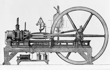
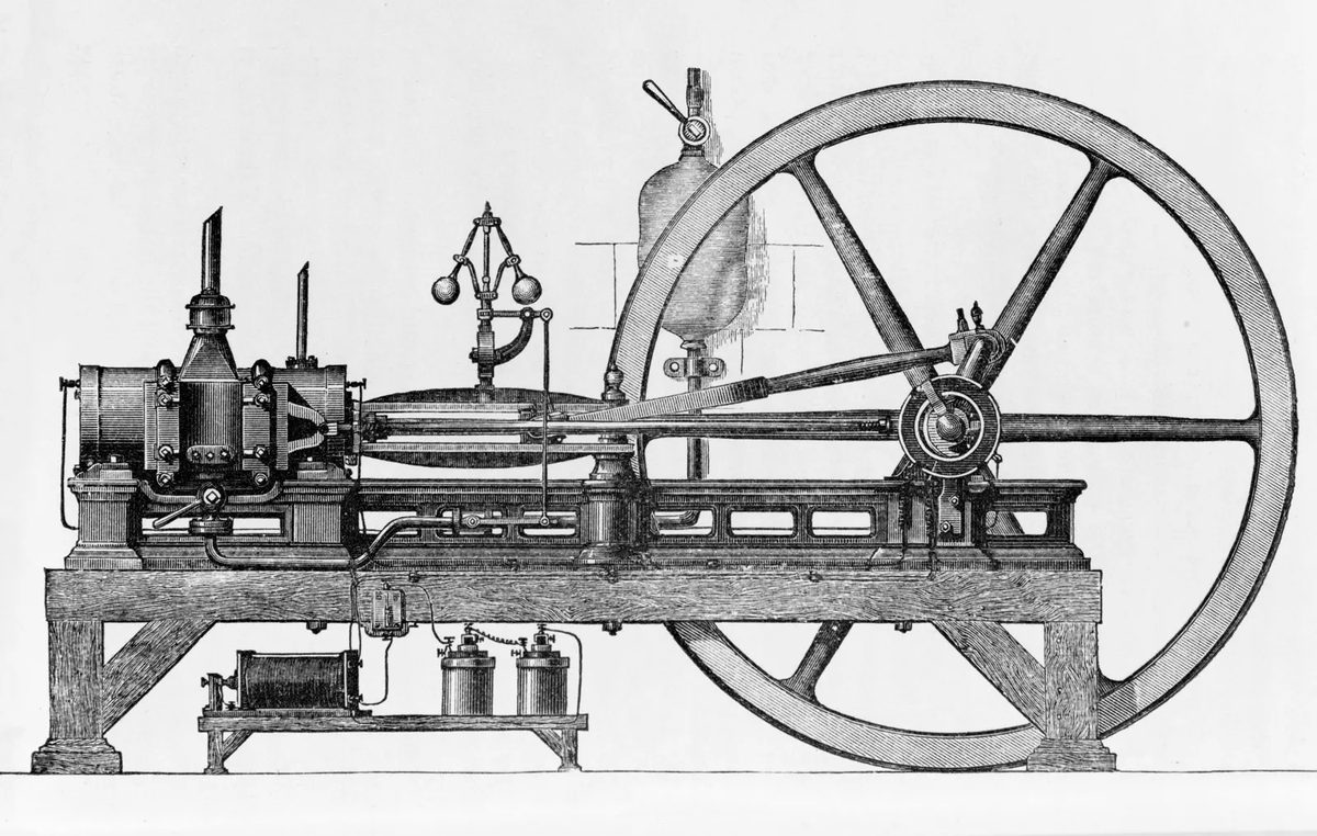
– The steam engine
– The gasoline engine
– The electric motor
– Standardization of parts
– The open-hearth furnace in steel
– The steam railroad
Lulls occur when innovation stalls. The average rate drops.
“A surge of labour-saving innovations would cause the overall average rate to move higher, while a technological lull would depress the average rate.”
How to read the data across sectors
Looking only at the national average misses the point. Growth is better understood by examining the relative contributions of individual industries. You need to look at why productivity changed in each specific sector.
Is it a new technology? A change in process? A shift in product mix?
Understanding these granular drivers matters. It tells you where the next wave of income growth will come from. It also highlights which sectors are stuck in low-productivity traps.
The data doesn’t lie, but it doesn’t tell the whole story until you break it down by industry.
How productivity metrics drive pay and planning
Productivity isn’t just a number on a spreadsheet. It acts as the ruler for efficiency in economic planning. When you need to forecast where an economy is heading, you look at output per worker or per machine. That yardstick sets the baseline. It also determines how much people get paid. If a factory runs on piecework, labor productivity is the sole determinant of wages. It grades workers who do similar tasks. It flags machines that are about to break down.
Developing countries use these metrics differently. They look at target productivity levels. They project labor force growth. They understand the link between capital per worker and output. This helps them estimate how much capital investment is required to hit those targets. It also helps estimate future job availability. If you know the probable annual gain in labor productivity and the probable annual increase in output, you can estimate how many jobs will open up.
Resource allocation follows these shifts. Resources flow to uses where they are most productive. When productivity changes over time, the pattern of use changes. An increase in labor productivity means fewer workers are needed per unit of output. That tends to reduce the demand for labor. But it also makes labor cheaper relative to other inputs. So there is a tendency to substitute labor for other factors.
When labor cost is a large part of total cost, a productivity increase pushes the price of the product down. Lower prices expand sales. That expands the demand for labor again.
The net result is complex. It depends on the sum of all these separate effects. It is not uncommon for the expansionary effects to predominate. Many economists consider that the normal outcome.
Why productivity growth fights inflation
Real average labor compensation has risen at about the same pace as labor productivity over the long run. This connection holds as long as the labor share of total cost remains stable. If nominal earnings grow faster than productivity, labor cost per unit of output rises. Prices rise too, unless profit margins shrink to compensate.
In general, prices rise by less than wage rates and other input prices when total productivity grows. Productivity growth is an anti-inflationary factor. Inflation is basically a monetary phenomenon, but productivity tempers it.
There is a significant negative correlation between relative industry changes in productivity and prices. When productivity rises, price tends to fall. In industries with significant price elasticity of demand, there is also a positive correlation between productivity and output. When productivity rises, output tends to rise. This is an interactive loop. Falling prices encourage more demand. Increased output enables economies of scale. Those economies of scale further enhance productivity.
How capital substitution affects employment trends
In dynamic economies, the supply of capital has risen faster than the size of the labor force. Wage rates have also risen faster than the price of capital. This creates a marked tendency to substitute capital for labor in almost all industries.
Does this mean mass unemployment? No. There has been no long-term trend toward increased unemployment. Real aggregate demand has risen enough to absorb the growth of the labor force. Cyclical fluctuations in output and employment in capitalist countries are not the result of technological displacements of labor. They reflect macroeconomic variables, such as the growth of the money supply, that affect aggregate demand.
Technology changes the mix. It does not necessarily shrink the pie. The money supply decides how much of the pie gets eaten.
How capital quantity and quality interact to drive output
Stop thinking of productivity as a single dial you can turn. It is a system. Labor, land, raw materials, capital equipment, and mechanical aids all feed into it. The education of the workforce, the specific technology in use, and how production is organized matter just as much. Even the cultural attitudes and psychological state of managers and workers shape the result.
These variables do not sit in isolation. They interact. In a high-productivity country, you typically see high technology, skilled workers, ample capital, and rational organization all at once. A low-productivity nation usually suffers from deficiencies across the board. Economists treat these factors like a system of simultaneous equations. No single variable holds causal priority. They act concurrently to shape the outcome.
Why technology and capital accumulation dominate long-term growth
When looking at changes over time, two factors stand out: technological change and capital accumulation. Everything else tends to play a subordinate, passive role. Why? Because substantial gains in productivity require new knowledge and the physical tools that embody it.
When technology advances, capital quality improves. More capital per worker usually follows. The types of raw materials might shift, with higher grades becoming necessary or lower grades becoming viable. Production methods change. While the transition from land to factory often brought hardship, and some technological advances made work more tedious, the dominant trend has been toward shorter hours and less arduous labor.
Reorganizing work or breaking down restrictive attitudes can yield dramatic, short-term gains. But those gains are limited. They are not sustainable engines. Technology and capital are the only factors that can drive large, systematic, and near-unlimited advances in productivity.
The diminishing returns of simple capital accumulation
Here is the trade-off. Just adding more of the same equipment does not yield proportionate output gains forever. If you keep adding identical tools, you hit a point where output per worker stops growing. Eventually, it declines.
This decline is far away for an economy with high technical knowledge but acute capital scarcity. But it is an ultimate certainty. The escape route is qualitative change. As knowledge and skill advance, capital instruments improve. This allows for continuous expansion without hitting the wall of diminishing returns. Data from broad sectors shows a rough correlation between the growth in capital per worker and increases in labor productivity. The key is not just more capital, but better capital.
Measuring productivity: The difficulty of input and output ratios
Before analyzing trends, you have to measure the ratio. This is harder than it looks.
Estimates of productivity rely on measuring output and input. Both components carry difficulties and limitations. Output is not always a single, clear number. Input is even trickier, because you are trying to quantify the combined effect of labor, capital, materials, and organization. The resulting estimates are approximations, not absolute truths.
Understanding these measurement constraints is essential. Without them, the data on productivity trends is just noise.
Why input-based estimates skew service sector productivity
The measurement problem gets worse when you move away from tangible goods. In most countries, the data on quantities and prices for finance and service industries is simply not there. So analysts take a shortcut. They estimate output changes by looking at input changes.
This is a bad trade-off for productivity math.
If you derive output from inputs, you artificially depress the real product estimate for the services sector. That downward bias ripples out, making the entire economy look less efficient than it actually is. You cannot use these proxy numbers for rigorous productivity measurement. They are approximations, not facts.
“Estimates so derived are not suitable for productivity measurement, however. They impart a downward bias to estimates of real product and productivity for the services sector.”
Quality changes make it harder still. When a product gets better, its price usually goes up. If you only measure physical volume, you miss the value added by that improvement. You see a higher cost per unit and assume inflation, not progress. For custom-built items like buildings, measurement methods have improved in recent years. But for nonmarket goods, like government services or household labor, you still have to fall back on input data. This is why productivity estimates usually stick to the private business sector. It is the only place where the data holds up under scrutiny.
How labor quality shifts distort raw headcounts
Labor input looks simple. Count the heads. Or, better, count the hours worked. But the data rarely captures what actually happens on the factory floor. Most official figures track hours paid, not hours worked. As paid holidays and leave expand, the gap between the two widens. If you use paid hours, you overstate the actual work done.
Even worse, standard estimates treat all workers as identical. They do not differentiate by skill level, industry, or occupation. Academic economists push back on this. They weight labor by occupation and industry, using average compensation from a base period as a proxy for value. This matters because the workforce changes over time.
Education rises. Training improves. Experience accumulates. A worker in 2024 is not the same economic unit as a worker in 1984. When you weight labor by these quality factors, the aggregate measure rises relative to the unweighted count. The difference between the two measures tells you how much of the productivity gain comes from a smarter, better-trained workforce. Ignoring that shift hides a key driver of economic performance.
Capital stock, utilization rates, and the value-added trap
Capital input is usually assumed to move in lockstep with real stocks of structures, equipment, inventories, and natural resources. Analysts weight these assets by their rates of return in a base period. That rate acts as a proxy for productivity.
But there is a trap. If you do not adjust for capacity utilization, the numbers lie. If a factory runs at 60% capacity one year and 80% the next, the productivity estimate will spike. That is not necessarily better technology or better labor. It is just more efficient use of existing assets. Some analysts adjust for this. Others leave it in, which means the productivity number reflects utilization swings rather than genuine efficiency gains.
Then there is the issue of intermediate goods. These are the materials, energy, and services consumed during production. In national income accounts, they cancel out. One industry’s output is the next industry’s input. So they are excluded from value-added calculations. But if you are comparing gross output, you have to count them. And when you do, you measure them the same way you measure final outputs: with constant unit values to strip out price changes.
Getting this right is not a technicality. It is the difference between seeing a real improvement in how an economy works and seeing a statistical artifact.
Why the late 19th century changed the math on wealth
The numbers get interesting around 1870.
For decades, labour productivity crawled. In Britain, starting around 1760, the average annual gain sat near 0.5 percent. The United States followed a similar slow burn until after the Civil War. That was the baseline. Then the curve bent.
By the latter part of the 19th century, Western Europe, the U.S., and Japan pulled ahead. The earlier leader, Britain, was actually outpaced. Look at real gross domestic product (GDP) per hour worked :
- Western European countries and Japan averaged 1.6 percent growth from 1870 to 1950.
- The United States hit 2 percent from 1870 to 1913.
- The U.S. accelerated to almost 2.5 percent between 1913 and 1950.
Canada, Australia, and smaller Western European nations tracked similar ranges. Meanwhile, most of the rest of the world was still waiting for that sustained lift in real per capita income.
Two percent sounds tiny. It isn’t. Compounded over a century, it multiplies output by more than seven times. That is the mechanism behind the massive expansion of living standards in industrialized nations.
What actually drove that acceleration?
It wasn’t just one invention. It was a stack of changes hitting at the same time.
Steam and internal-combustion engines reshaped transportation. The telephone and wireless communication rewired how information moved. Together, they expanded trade, both domestic and international. Britain’s free trade model nudged other countries toward liberalization, opening markets that had been closed.
Corporate behavior shifted, too. Large companies started running purposeful research and development programs. Invention stopped being a fluke and became a budget line.
Education kept pace. Business schools opened to teach management as a discipline. As per capita income rose, saving rates went up with it. That higher saving rate fueled investment in new plants, equipment, and natural resource development.
Agricultural productivity improved. Labour mobility increased. Those two factors allowed manufacturing to scale massively, eventually giving way to the service industries we rely on today.
The compounding effect of 1.6 to 2.5 percent annual growth isn’t just a historical footnote. It is the baseline expectation for any economy that wants to avoid stagnation. If your portfolio, business, or career plan doesn’t account for that kind of long-term compounding, you are planning around a world that stopped existing in 1900.

How global productivity accelerated after World War II
The postwar era marked a massive shift in how economies functioned. In the five major industrialized nations, labor productivity growth tripled between 1950 and 1973 compared to the previous eight decades. This surge wasn’t just a U.S. phenomenon. In twelve other industrialized countries, real GDP per employed person grew at an average rate of about 4 percent annually during that same window. That figure was roughly double the rate seen in the United States.
Then the 1970s hit. Productivity growth dropped by almost half in those five major economies. The deceleration was steeper in the U.S., where growth slowed to virtually zero between 1973 and 1979. By the late 1970s, the 12-nation average had fallen to 2.2 percent per year.
But the story doesn’t end there. After 1981, the U.S. rate accelerated significantly. The 12-nation average continued to slide, settling at 1.8 percent. Even then, it remained well above the U.S. rate of 0.8 percent per year.
Why convergence happened among industrialized nations
A clear pattern emerged in the data: industrialized nations were converging. In 1950, the average real GDP per person for 11 industrialized countries was about 44 percent of the U.S. level. By 1986, that figure climbed to almost 80 percent.
This wasn’t random. There is a significant negative correlation between starting levels and growth rates. Countries that began farthest behind in 1950 grew most rapidly in productivity through 1986. This tendency toward convergence existed before 1950, but it became much stronger during the golden quarter-century following World War II.
The postwar period was a watershed. Most nations outside the original industrialized group began recording substantial increases in labor productivity starting around 1950.
Fragmentary data suggests low productivity growth was the norm for many of these nations before 1950. After the immediate postwar reconstruction period, most were able to accelerate their gains markedly.
Which countries saw the fastest productivity gains?
Global data shows some convergence within groups, but not worldwide. Low-income countries had the lowest rates of productivity advance. Oil exporters and relatively industrialized middle-income countries saw the highest rates.
Centrally planned economies tell a mixed story. From 1950 to 1970, they recorded above-average rates of productivity growth. After 1970, those rates fell below the average.
How international policy fueled the postwar productivity surge
The global upsurge in productivity wasn’t accidental. It reflected a deliberate shift toward internationalist thinking and policy-making among developed nations.
Several mechanisms drove this change:
- The creation of the World Bank and the International Monetary Fund encouraged cooperative economic and financial relationships.
- The Marshall Plan, an outgrowth of the Cold War, launched a major U.S. effort to aid reconstruction and economic development in the noncommunist world.
- The plan included the creation of productivity centers in member countries. These centers sent teams to the United States to study and facilitate the transfer of advanced technology.
- Private lending abroad was encouraged alongside loans from the World Bank and other international institutions.
- Regional trade associations formed to reduce trade barriers among members.
- The General Agreement on Tariffs and Trade (GATT) promoted broader liberalization of international trade.
As a result, world trade grew even faster than production. Crucially, this trade included transfers of advanced machinery and other producer goods from the United States and other industrialized countries. Those transfers helped raise the productivity of the purchasing countries.
The mechanism is straightforward: access to better tools and technology boosts output per worker. The postwar institutions made that access possible on a scale never before seen. Whether the benefits will persist or fade depends on factors the data doesn’t fully reveal. What’s clear is that the 1950 to 1973 period remains an outlier in modern economic history.


How developing nations absorbed industrial secrets
The flow of expertise did not stop at borders. Multinational corporations, mostly U.S.-based, moved more than just money into host countries. They brought managerial skills, technical know-how, and training programs that placed local nationals in upper-level positions. Patent licensing opened another door. As more students from developing nations enrolled in American universities, particularly in business and engineering, they carried that institutional knowledge back home. Professional associations and journals kept the pipeline open.
Why Japan and Europe closed the gap
Between 1950 and 1973, the productivity distance between the United States and other industrialized nations shrank. The driver was capital formation. Japan saved nearly one-third of its GDP. Western Europe saved about one-fourth, helped by tax laws that encouraged it. The U.S. saved roughly half what Japan did.
That disparity mattered. Higher saving rates meant more private and public investment. The average age of equipment and structures in those countries dropped rapidly. Trade grew, allowing firms to achieve economies of scale. Labor shifted out of low-return sectors like agriculture and self-employment.
When a country saves more than it consumes, it builds the physical capital that outproduces competitors with older factories.
The cost of catching up
Once other nations reached parity in technology, the dynamic changed. After 1960, catching up became harder. Why? Because transferring technology from abroad is cheaper than developing it from scratch. Once a country approaches the frontier, it must invest in its own R&D. That investment is expensive. As a result, productivity growth rates tended to converge.
This convergence is not a failure. It is a mathematical inevitability. The easier gains come from adopting existing methods. The harder gains require original innovation.
The 1973-1979 productivity shock
The slowdown after 1973 was not unique to any single country. It was almost universal. Two oil price shocks, in 1973 and 1979, accelerated inflation. Inflation reduced economic profits. Lower profits meant lower saving and investment rates.
Several structural factors compounded the problem:
- Energy-intensive equipment became obsolete overnight.
- Growth in real R&D spending slowed.
- The pace of technological innovation dropped.
- The benefits of shifting labor between industries diminished.
- Demographics worked against growth. The changing age and sex mix of the labor force reduced short-run productivity, especially in North America.
- Government regulations on environment, health, and safety increased in the 1970s. These rules raised costs and inputs without a proportional increase in measured output.
Why the U.S. recovered while others did not
In the 1980s, the United States reversed many of those negative trends. Productivity growth accelerated. Other industrialized countries did not see the same bounce. The difference likely came down to technology transfer. The flow of new methods and techniques from the U.S. to other advanced economies probably declined.
Developing countries with enough absorptive capacity continued to improve. They still had room to adopt foreign technology. For them, the frontier was further away. The cost of catching up remained low.
There is no reason to assume that advantage will last forever, but it did hold through the period covered here. The trade-off is clear. Fast growth comes from borrowing other people’s ideas. Slower, more expensive growth comes from creating your own.


